Google recently released the Gemma 3n models — E4B and E2B. The models are packed with novel components and features from PLEs, ASR and AST, MobileNet-V5 for vision etc. But one of the more interesting parts in the announcement is that E2B isn’t just a smaller sibling trained separately (or distilled) like other family of models we have previously seen (7B, 11B, 70B etc) — it’s actually a sub-model within E4B. Even more intriguing, the release mentioned that it’s possible to “mix and match” layers between the two, depending on memory and compute constraints to create even more models of different sizes. How was such a modularity achieved? How are different sized models trained simultaneously?
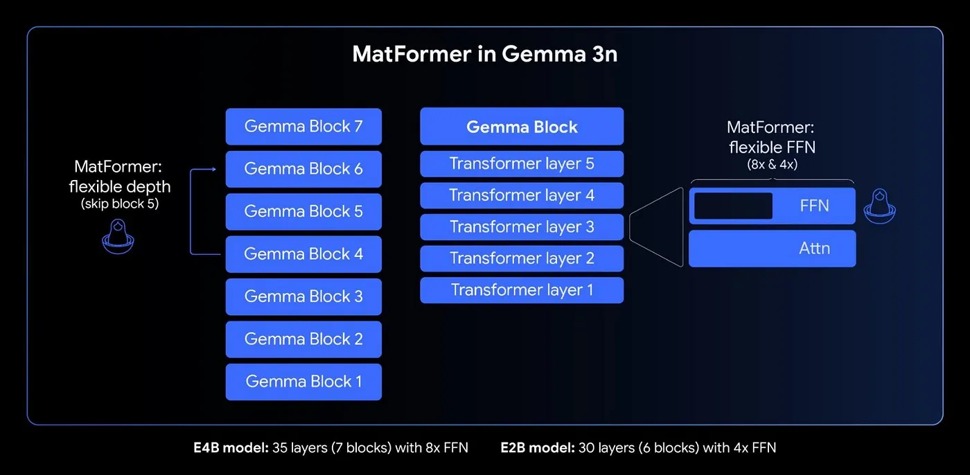
It turns out Gemma 3n uses an architecture called MatFormer — short for Matryoshka Transformer — (DeepMind, NeurIPS 2024). The idea is surprisingly elegant: train a larger model (E4B) in such a way that smaller, fully functional sub-models (like E2B) are embedded inside it. Like nested Matryoshka dolls, except here, it’s transformer layers. No distillation. No retraining. No routing like mixture of experts. Just shared weights and slicing while still preserving effective accuracy.
In this post, we’ll go deep into how MatFormer works — what parts of the architecture are shared, how sub-models are extracted, what makes the training objective feasible, and why this changes how we think about model scaling and deployment, especially for constrained environments.
MatFormer — Matryoshka Transformer
A standard transformer layer consists of two learnable blocks — projections matrices in the Multi-head self-attention and the Feed-forward network (FFN). Feed-forward networks (FFNs) are the dominant contributors to both the parameter count and inference latency, and Matformer papers presents most of its experiments by applying the proposed nested architecture to FFN block (though it can be applied to any learnable weight).
In large-scale language models like Llama 3 and Gemma 3, the Feed-Forward Network (FFN) within each transformer block is typically implemented as a two-layer MLP (Gated MLP):
- First Linear Layer (Expansion/Intermediate): Projects the input embedding to a higher-dimensional hidden space.
- Activation Function: Often uses GELU, ReLU, or more recently, gated variants like SwiGLU or SiLU.
- Second Linear Layer (Projection): Projects the hidden representation back to the original embedding dimension
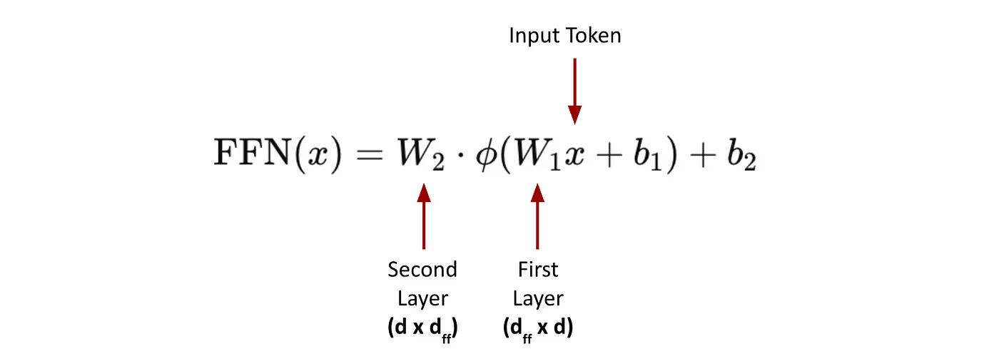
Here $d$ is token embedding dimension (model dimension). $d_{ff}$ is the Feed-forward hidden dimension. It’s the size of the intermediate activation in the FFN (feed-forward network) block. It’s typically much larger than $d$ ($d$ » $d_{ff}$), usually 4x–6x as large. For example, in a LLaMA-style transformer with $d$ = 4096, FFN often uses $d_{ff}$ = 11008 or more. These layers dominate model size and memory usage.
Nested multiple FFN widths from one FFN:
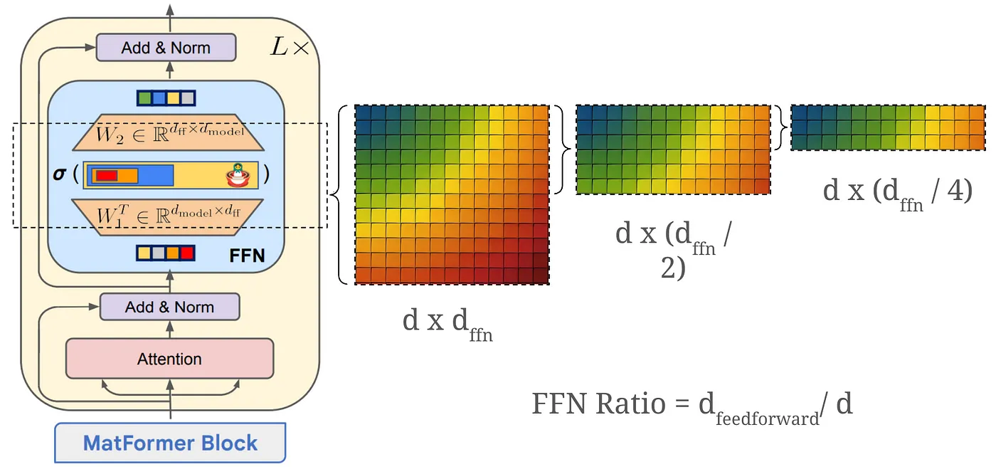
Instead of fixing a single FFN width per layer, MatFormer nests multiple FFNs of different widths inside each transformer block.
Let $d_{ff}$ be the largest FFN width we want to support (e.g. 16384), then sub-models with FFN width m_i simply use the top-left submatrix of the full weight matrices.
For example, let’s say $d$ = 4096 (input token dimension) and d_ff = 16384 (full FFN hidden dimension) and we choose a set of granularities we want to train for: m1 = 4096, m2 = 8192, m3 = 12288 and m4 = 16384. Here the idea is that submodules of smaller widths are subsets of those with larger widths.
Training All Granularities Jointly
The next question is: how do we make sure all sub-models perform well? Rather than jointly computing the loss across all submodels in each training step, MatFormer adopts a more efficient approach: stochastic sampling of submodel granularities during training.
MatFormer uses a multi-granularity loss, computed as:
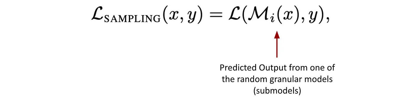
$M_i$ is the submodel corresponding to the i-th granularity (i.e., using only the first $m_i$ neurons in each FFN).
This design has two critical benefits. Only one submodel is evaluated per step, avoiding the overhead of computing all granularities simultaneously. Additionally, since each submodel shares parameters with the larger model, training a different one in each step still updates the shared weight matrices.
In the paper they uniformly sample each submodel with equal probability while computing this loss.
In the experiments in appendix of the matformer, authors experiment with tuning the sampling probabilities for individual granularities. They find that upweight the loss for the largest granularity gives boost to the performance of bigger models while modest degradation to the performance of the smaller submodels.
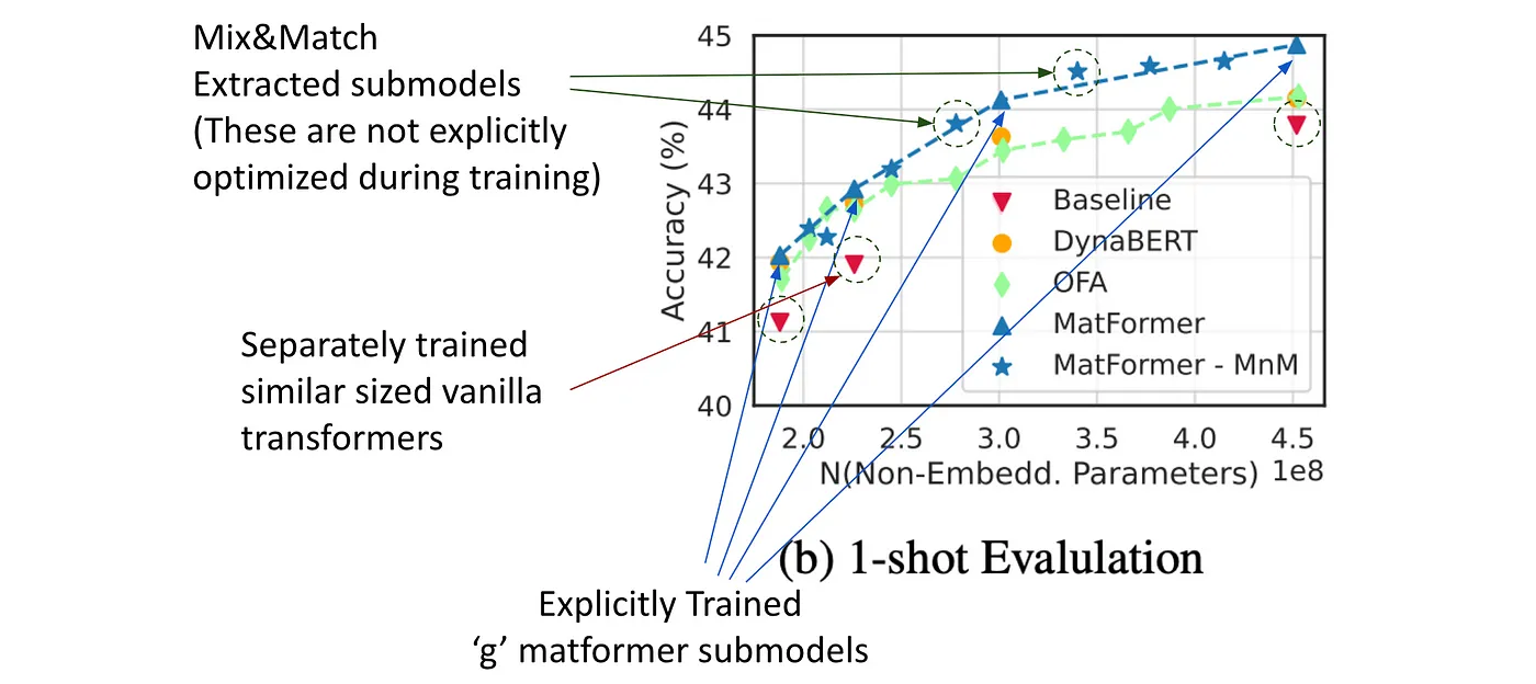
Way more number of accurate smaller models for free (Mix’n’Match)
One of the most interesting aspects of MatFormer is that it doesn’t just give you g (number of trained) nested submodels — it gives you hundreds of submodels for free at inference time via a simple technique called Mix’n’Match.
During training, MatFormer explicitly optimizes $g$ submodels, each corresponding to a specific granularity (i.e., FFN width) across all layers. For example, one submodel might use width $m_1$ (e.g., 4096) in all layers, another might use $m_3$ (e.g., 12288) everywhere. But this doesn’t restrict us to uniform widths during inference.
At inference time, we can vary the FFN width layer by layer — one layer could use $m_2$, the next $m_3$, the next $m_2$ again, and so on. Since all the FFN blocks are nested, these hybrid models require no retraining, no fine-tuning, and no architectural redefinition.
This layer-wise configuration space is huge — for L layers and g granularities, there are g to the power L possible submodels. Even for small values (e.g., 32 layers, 4 granularities), that’s billions of options.
But not all of these perform equally well. To select a good configuration, the authors propose a simple heuristic:
Prefer submodels where FFN widths vary slowly and consistently across layers.
In other words: Avoid large jumps between small and large granularities from one layer to the next.
Also, favor monotonic or gently increasing sequences — e.g., use m_2 for early layers and gradually grow to m_3 in later layers.
this heuristic aligns well with how the model was trained — where sampled submodels always used uniform widths per step. So while hybrid layer-wise combinations were never explicitly trained, configurations that look similar to the training regime generalize better.
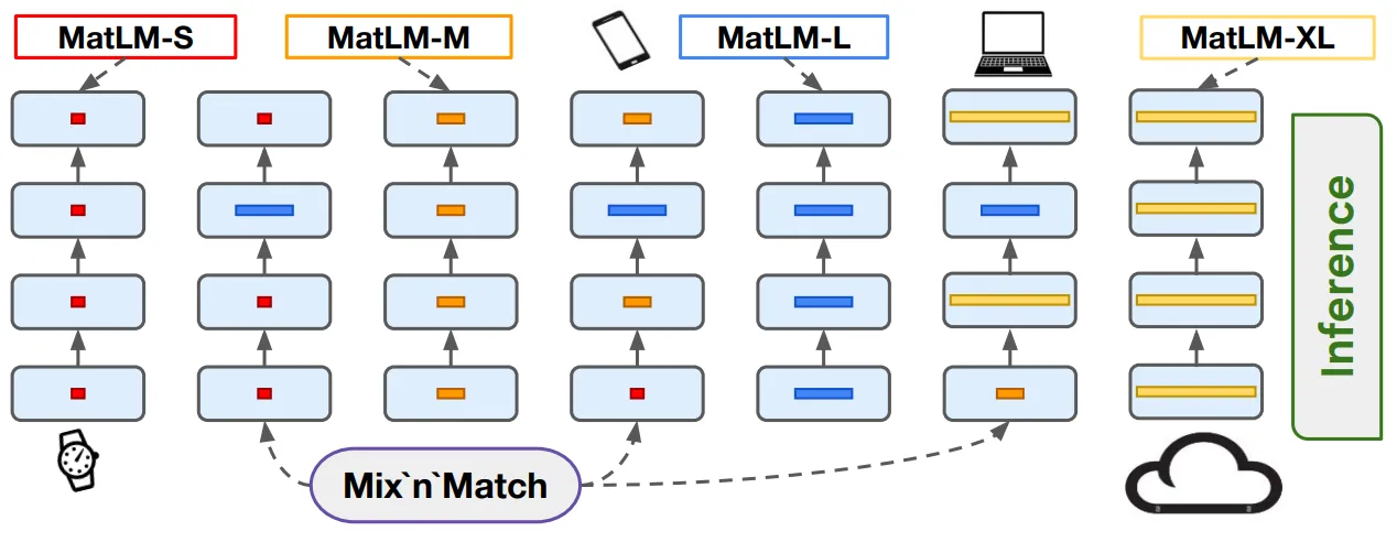
The authors of Matformer applied this approach to two transformer based models — LLMs and ViTs (called MatLM and MatViT respectively)
For LLMs trained with Matformer’s nested FFN, the authors find that all granularity submodels of Matformer outperform their respective separately or independently trained similar sized vanilla transformers LLMs. In above the experiments for MatLM, they trained 4 nested granularities with $d_{ffn}$ (FFN dimension) / $d$ (model dimension) ratios of → {0.5, 1, 2, 4}. They named respective models as S, M, L and XL. Here XL is the full model.
Even though in the matformer paper the maximum size transformer trained was 850M parameters, Gemma 3n utilizing matformer for 4B (effective 5B) shows parametric scalability of this approach.
Performance of Mix’n’Match models
They also observed that Mix’n’Match models tend to lie on the accuracy-to-compute trade-off curve (Pareto-optimal accuracy-vs-model-size). Which means that based on the available compute resources, the biggest possible Mix’n’Match model can be created during inference, which showed likely have better accuracy then relatively smaller trained submodel. This has interesting implications. For instance, many a times in deployment use-cases we have enough compute resources (GPU memory) to load a 20B parameter model, but the nearest variant that is available to us is either a 14B or 33B. Using the 14B parameter models leads to underutilization of resources and subpar performance and the 33B parameter model won’t fit in memory. This Mix’n’match approach allows to create nearly perfect sized variants for free with commensurate accuracy trade-off.
Gemma 3n being based on the Matformer architecture also gives us the liberty to perform Mix’n’Match and create many more model sizes between 2B and 4B. In terms of the performance, Gemma 3n E4B has MMLU accuracy of 62.3%, and E2B has 50.90%. Mix’n’Match ‘ed variants such as 2.54B has MMLU accuracy of 55.40% and 2.69B has 57.70%, which significantly better than 2B and little lower than 4B. This allows us to get perfectly sized accurate model for on-device deployment usecase — smartphone, tab, mac, etc.
To try out creating mix’n’match variants of the Gemma 3n model, Gemma 3n team has released Matformer Lab, which is colab notebook where you can slice the model and push it to huggingface. They have also released some optimal slicing configurations (as we saw above though we can generated g to the power L models, not all mix’n’matches might be optimal for desired size) on hugging face — google/gemma3n-slicing-configs. These configurations include varying the FFN dimension at either layer level, which is more finegrained or at block level which includes 4 local layers and 1 global layer.
Another aspect of training smaller models as nested submodels of the bigger model that authors focus on is consistency of predicted tokens. One way verifying this consistency is by looking at rejection rates of speculative decoding. In speculative decoding, instead of always autoregressively predicting the tokens from the large target model, there is a smaller “Draft model” and a larger “Verifier model” (target model). The draft model performs token speculation, i.e. it predicts the next n tokens along with their probabilities, and the target model parrallely performs verification of the predicted tokens. Comparing the target model’s probabilities for the same tokens predicted by the draft model rejection sampling is performed. When the draft models is significantly off with respect to the target model, the draft model’s predictions are rejected. As one could see, here the most significant speed-ups come when the draft model consistently predicts the similar token distribution as the target model, leading to lesser rejections. If rejections would be more, then we won’t get the desired inference speed ups expected from speculative decoding. Authors of Matformer, show that since the smaller submodels are nested within and are trained along side the larger (XL) model they show more consistent nature required for drafter and verifier models. When traditional speculative decoding using a independently trained “S” sized model with XL model as target led to 10% inference speed time speedup over autoregressive decoding of target model, using the “S” sized MatLM model led to 16% speedup.
Moreover since the two MatLM models (S and XL) are trained together, it allows for shared attention caches (this cannot be done with indepedently trained models since the latent reps would be very different).
What I find even more interesting is that during deployment, the universal XL model can be stored in memory and based on the compute constraints be used to extract an adaptable smaller model. This dynamic resource adaptive model extraction and inference might be really useful for edge use-cases.
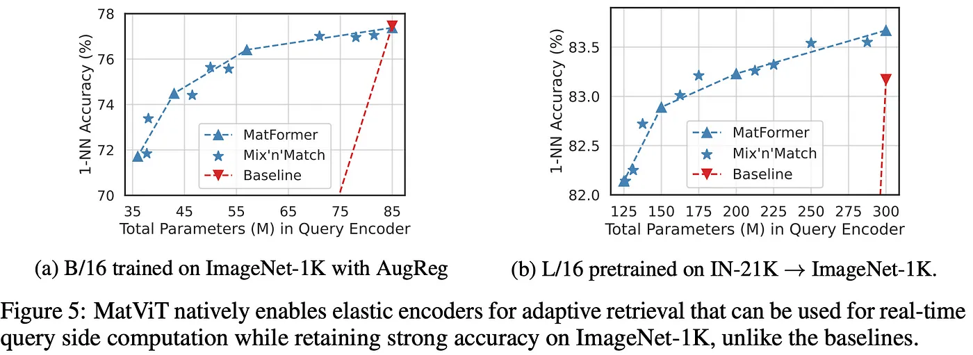
The Case for Image Retrieval
Authors also trained the Matformer for ViTs (Vision transformers) encoders (MatViT). Apart from similar trends as observed for MatLM, an interesting use-case of MatViT is in fast image retrieval. In typical image retriveal, getting embeddings for gallery images (gallery creation) happens offline and are stored, while quering (creating embedding for the query image) happens real-time. This means that gallery embeddings can utilize bigger more accurate models, while the query embeddings might require a smaller model for fast inference. Since smaller submodels in Matformers are nested and trained jointly, they tend to share the same embedding space as the bigger model and lead to meaningful distances for nearest neighbour based retrieval. This allows for using the XL model for gallery encoding, while using a smaller (ex: S) model for querying.
How are MatFormers different from MoEs?
Almost all major recent open LLM transformers are MoE architectures. Mixture of Experts (MoE) models increase capacity by adding multiple FFNs — called experts — to each transformer layer. At inference time, a router decides which expert(s) to use for each token, and only those selected paths are executed. This reduces compute cost per forward pass, since most experts stay inactive. However, all expert weights still need to be loaded into memory, because the router can choose any of them at runtime. This makes MoE models difficult to deploy on memory-constrained devices — while compute is sparse, memory usage stays high. In contrast, MatFormer doesn’t rely on routing or multiple experts. Instead, each FFN is designed to support multiple granularities by nesting smaller sub-networks inside larger ones. At inference time, a specific submodel can be selected and run independently. Only the parameters for that submodel need to be loaded into memory. This makes MatFormer much better suited for on-device or low-memory inference, where storing the full model isn’t feasible.
Conclusion
MatFormer represents a significant shift in how we approach model training, inference, and deployment. Traditionally, large models are trained with massive compute budgets, and smaller variants are created afterward — either trained separately or distilled from the larger ones. MatFormer breaks from this pattern by nesting multiple functional submodels within a single transformer via shared weight training, eliminating the need for costly distillation, retraining, or complex routing like Mixture-of-Experts. This design unlocks a smooth continuum of resource-adaptive models — from lightweight, mobile-ready deployments to full-capacity inference engines — all derived from a single base model. The success of Gemma 3n’s E2B and E4B, the versatility of Mix’n’Match variants, and the cross-modal generalizability demonstrated by MatViT encoders suggest that MatFormer-style architectures could become the new default for how research labs release scalable model families.
Resources
- Matformer: Devvrit, Fnu, et al. “Matformer: Nested transformer for elastic inference.” Advances in Neural Information Processing Systems 37 (2024): 140535–140564. https://arxiv.org/abs/2310.07707
- Speculative Decoding: Leviathan, Yaniv, Matan Kalman, and Yossi Matias. “Fast inference from transformers via speculative decoding.” ICML, PMLR, 2023 https://arxiv.org/pdf/2211.17192
- NeurIPS 2023 video and slides: https://neurips.cc/virtual/2023/80908
- Gemma 3n Developer Guide: https://developers.googleblog.com/en/introducing-gemma-3n-developer-guide/
- Hugging Face Blog: https://huggingface.co/blog/gemma3n
- MatFormer Lab: [https://colab.research.google.com/github/google-gemini/gemma-cookbook/blob/main/Gemma/Gemma_3n]MatFormer_Lab.ipynb
- Gemma 3 Technical Report: https://arxiv.org/pdf/2503.19786v1
Footnote on Gemma 3 attention: See Gemma 3 technical paper for details on global and local attention
Subscribe at the bottom of this page to get updated when a new article comes up!